The rule of thumb for equity investments is to not time the market, but there are also several analyses correlating investing at high index PE levels with lower returns. So can we use the PE levels of indices to generate better returns than SIP and reduce volatility of the portfolio?
DISCLAIMER: This is for informational purposes only and cannot be considered as financial advice. I cannot be held liable for the outcome of any action taken as a result of reading the information contained here. Please contact a certified financial adviser before making investment decisions.
Unlike fixed deposits, equities do not compound at a fixed rate. However, compounding is just the process of earning returns on previously earned returns. So rather than using PE just to time the investments, let us also use it to book some profits when we deem the market is over-valued and re-invest when under-valued.
Let us assume a monthly investment of ₹10,000 and simulate the management of equity and cash components in the portfolio using different strategies, from 1 April, 2006 to 30 April, 2017. We never sell any unit within a year of buying it, to avoid STCG.
Equity units are bought when the PE of either Nifty 50 or Nifty 500 is below 16 and units older than a year are sold when PE of both indices is above 23. When PE is between 16 and 23, additional investments are held as cash.
Equity units are bought when the PE of either Nifty 50 or Nifty 500 is below the median of preceding 5 years and units older than a year are sold when PE of both indices is above the 90th percentile of preceding 5 years. When PE is between the median and 90th percential, additional investments are held as cash.
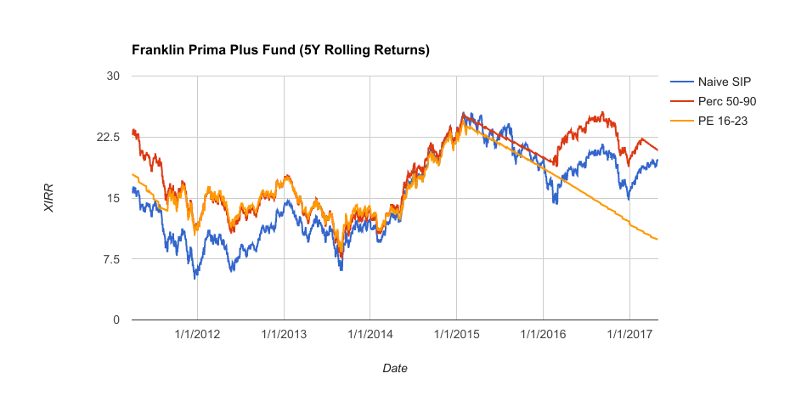
Let us compare the 5-year rolling returns of SIP with the above strategies and see how they fare. I have chosen 3 actively managed multi-cap funds instead of index returns, to see the impact of active management.
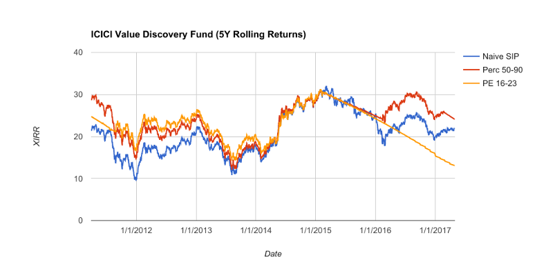
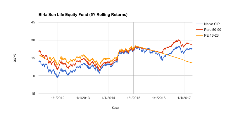
The magnitude of impact differs by fund, but some common patterns emerge. Both strategies beat returns from SIP until 2016, but using absolute PE levels leads to staying out of the market for too long during prolonged over-valuation. Using relative PE levels avoids this by re-entering the market during crash of 2016. I tried with different buy levels for absolute PE, but none of them did better than relative timing.
The table below gives the XIRR and the final value of corpus for SIP and timing by relative PE levels at the end of the entire 11-year duration.
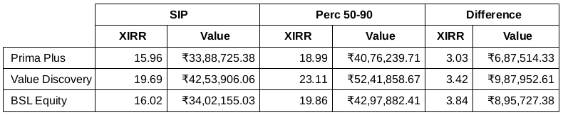
Timing with relative PE beats SIP in all 3 cases with a difference of whopping 7-10 lakhs in final corpus and 3-4% in XIRR!
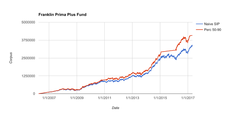
Timing has prevented the corpus from falling in the beginning of 2011 and in 2015. These appear to be the primary contributors of outperformance. While not visible in the chart, the corpora began to diverge as early as 2008.
I did not simulate every possible combination of PE level, but I did try out a few other levels for both absolute and relative PE. These two happened to generate the best return among those.
So far timing with relative PE levels sounds great, but a major drawback of back-testing with Indian indices is that they are too young. So what happens when we try this on S&P 500?
I downloaded the S&P 500 data from here. Unlike Nifty, we only have monthly data here. I also changed the rolling returns duration to 10 years, to see the impact for long-term investors.
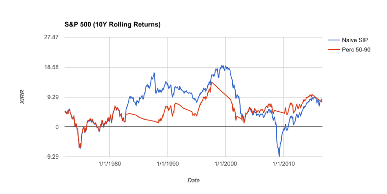
There is a stretch of 20 years where SIP has beaten timing with relative PE! The volatility is lower when timing, but the opportunity cost can be huge depending on the period we look at.
Markets can remain irrational longer than you can remain solvent. There is no reason to expect Indian market to behave differently in future from how the US market has behaved in the past. It is best to stick to an asset allocation appropriate for our financial goals, rebalance periodically, and reduce equity exposure as we get closer to the goals.
All opinions are my own. Copyright 2005 Chandra Sekar S.